序列数据概述
序列数据是指按时间顺序排列的数据,其中每个数据点都依赖于前面的观测值。序列模型的核心是估计条件概率分布:
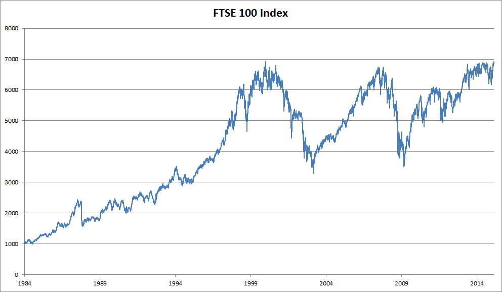
图 1:富时 100 指数 - 典型的序列数据示例
序列数据的特点
- 时间依赖性:当前观测依赖于历史信息
- 因果性:未来不能影响过去
- 非平稳性:数据分布可能随时间变化
- 预测难度:外推比内插更困难
序列模型的挑战
- 输入维度变化:历史观测序列长度不固定
- 误差累积:多步预测中错误会快速积累
- 计算复杂度:处理长序列计算量大
序列建模策略
自回归模型
基于历史观测值来预测未来值:
两种主要策略:
flowchart TD
    A[序列建模策略] --> B[截断历史]
    A --> C[隐状态建模]

    B --> B1[固定窗口τ]
    B --> B2[马尔可夫假设]

    C --> C1[隐变量h_t]
    C --> C2[递归更新]

    style A fill:#FF4444,stroke:#FFFFFF,stroke-width:3px,color:#FFFFFF
    style B fill:#00CCFF,stroke:#FFFFFF,stroke-width:3px,color:#FFFFFF
    style C fill:#00FF88,stroke:#FFFFFF,stroke-width:3px,color:#000000
    style B1 fill:#FFB347,stroke:#000000,stroke-width:2px,color:#000000
    style B2 fill:#FFB347,stroke:#000000,stroke-width:2px,color:#000000
    style C1 fill:#98FB98,stroke:#000000,stroke-width:2px,color:#000000
    style C2 fill:#98FB98,stroke:#000000,stroke-width:2px,color:#000000
简单例子:股票价格预测
- 假设今天股价为 100,昨天为 95,前天为 98
- 自回归模型:
- 预测明天价格可能为 102 或 97
马尔可夫模型
假设当前状态只依赖于前 τ 个观测:
一阶马尔可夫链:
其中
简单例子:天气预测
- 状态:{晴天, 雨天, 阴天}
- 一阶马尔可夫假设:今天天气只依赖昨天
- 转移概率:
- P(今天晴天 | 昨天晴天) = 0.7
- P(今天雨天 | 昨天晴天) = 0.2
- P(今天阴天 | 昨天晴天) = 0.1
- 如果昨天是晴天,今天最可能还是晴天
隐变量自回归模型
保持历史信息的总结

图 2:隐变量自回归模型架构
简单例子:RNN 语言模型
- 输入序列:["我", "爱", "学习"]
- 隐状态更新:
→ 记住"我"的信息 → 记住"我爱"的信息 → 记住"我爱学习"的信息 - 预测下一个词:
可能是"编程"、"数学"等
flowchart LR
    x1[我] --> h1[h₁]
    h0[h₀] --> h1
    h1 --> h2[h₂]
    x2[爱] --> h2
    h2 --> h3[h₃]
    x3[学习] --> h3
    h3 --> y[预测:编程]

    style x1 fill:#FF6B6B,stroke:#FFFFFF,stroke-width:2px,color:#FFFFFF
    style x2 fill:#FF6B6B,stroke:#FFFFFF,stroke-width:2px,color:#FFFFFF
    style x3 fill:#FF6B6B,stroke:#FFFFFF,stroke-width:2px,color:#FFFFFF
    style h1 fill:#4ECDC4,stroke:#FFFFFF,stroke-width:2px,color:#FFFFFF
    style h2 fill:#4ECDC4,stroke:#FFFFFF,stroke-width:2px,color:#FFFFFF
    style h3 fill:#4ECDC4,stroke:#FFFFFF,stroke-width:2px,color:#FFFFFF
    style y fill:#FFD93D,stroke:#000000,stroke-width:2px,color:#000000
序列建模的数学基础
三种模型对比
flowchart TD
    A[序列模型对比] --> B[自回归模型]
    A --> C[马尔可夫模型]
    A --> D[隐变量模型]

    B --> B1[使用全部历史]
    B --> B2[计算复杂度高]
    B --> B3[表达能力强]

    C --> C1[固定窗口大小]
    C --> C2[计算简单]
    C --> C3[独立性假设]

    D --> D1[压缩历史信息]
    D --> D2[递归更新]
    D --> D3[平衡复杂度]

    style A fill:#FF1744,stroke:#FFFFFF,stroke-width:3px,color:#FFFFFF
    style B fill:#FF9800,stroke:#FFFFFF,stroke-width:3px,color:#FFFFFF
    style C fill:#2196F3,stroke:#FFFFFF,stroke-width:3px,color:#FFFFFF
    style D fill:#4CAF50,stroke:#FFFFFF,stroke-width:3px,color:#FFFFFF

    style B1 fill:#FFE0B2,stroke:#000000,stroke-width:2px,color:#000000
    style B2 fill:#FFE0B2,stroke:#000000,stroke-width:2px,color:#000000
    style B3 fill:#FFE0B2,stroke:#000000,stroke-width:2px,color:#000000

    style C1 fill:#BBDEFB,stroke:#000000,stroke-width:2px,color:#000000
    style C2 fill:#BBDEFB,stroke:#000000,stroke-width:2px,color:#000000
    style C3 fill:#BBDEFB,stroke:#000000,stroke-width:2px,color:#000000

    style D1 fill:#C8E6C9,stroke:#000000,stroke-width:2px,color:#000000
    style D2 fill:#C8E6C9,stroke:#000000,stroke-width:2px,color:#000000
    style D3 fill:#C8E6C9,stroke:#000000,stroke-width:2px,color:#000000
联合概率分解
前向分解:
后向分解:
静态性假设
假设序列的动力学规律不随时间改变,即分布是平稳的:
马尔可夫链的边际化
对于二阶马尔可夫链:
预测方法与挑战
预测类型
flowchart LR
    A[预测方法] --> B[单步预测]
    A --> C[多步预测]

    B --> B1["x̂t+1 = f(xt, ..., xt-τ+1)"]
    C --> C1[逐步预测]
    C --> C2[误差累积]

    style A fill:#9B59B6,stroke:#FFFFFF,stroke-width:3px,color:#FFFFFF
    style B fill:#2ECC71,stroke:#FFFFFF,stroke-width:3px,color:#FFFFFF
    style C fill:#E74C3C,stroke:#FFFFFF,stroke-width:3px,color:#FFFFFF
    style B1 fill:#58D68D,stroke:#000000,stroke-width:2px,color:#000000
    style C1 fill:#F1948A,stroke:#000000,stroke-width:2px,color:#000000
    style C2 fill:#F1948A,stroke:#000000,stroke-width:2px,color:#000000
单步预测公式:
k 步预测
对于观测序列直到
多步预测的递归公式
误差累积问题
假设第一步误差为
- 第二步误差:
- 误差快速累积,导致长期预测质量下降
误差累积可视化
flowchart LR
    A[真实值] --> B[1步预测]
    B --> C[2步预测]
    C --> D[3步预测]
    D --> E[4步预测]

    A --> A1[x₁ = 10]
    B --> B1[x̂₂ = 10.1<br/>误差=0.1]
    C --> C1[x̂₃ = 10.3<br/>误差=0.3]
    D --> D1[x̂₄ = 10.7<br/>误差=0.7]
    E --> E1[x̂₅ = 11.5<br/>误差=1.5]

    style A fill:#00C851,stroke:#FFFFFF,stroke-width:3px,color:#FFFFFF
    style B fill:#FF6D00,stroke:#FFFFFF,stroke-width:3px,color:#FFFFFF
    style C fill:#FF6D00,stroke:#FFFFFF,stroke-width:3px,color:#FFFFFF
    style D fill:#FF1744,stroke:#FFFFFF,stroke-width:3px,color:#FFFFFF
    style E fill:#FF1744,stroke:#FFFFFF,stroke-width:3px,color:#FFFFFF
总结
- 时序模型中,当前数据跟之前观察到的数据相关
- 自回归模型使用自身的过去数据来预测未来
- 马尔科夫模型假设当前只跟最近少数数据相关,从而简化模型
- 潜变量模型使用潜变量来概括历史信息
- 预测方法包括单步预测和多步预测,但多步预测面临误差累积问题
参考资料:D2L 序列模型