![]()
传统的 RNN 网络
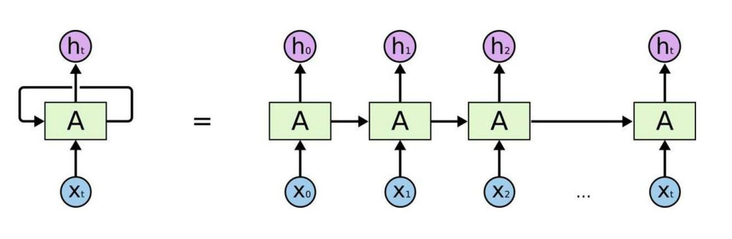
传统的 RNN 计算时有什么问题?
长期依赖问题
- 在处理长文本序列时,RNN 无法有效记住前面的序列信息
- 随着序列长度增加,早期信息会逐渐丢失
梯度消失/爆炸问题
- 在反向传播过程中,梯度可能会指数级衰减(梯度消失)
- 或者梯度可能会指数级增长(梯度爆炸)
- 导致网络难以学习长距离依赖关系
顺序计算限制
- RNN 必须按顺序处理序列,无法并行计算
- 训练和推理效率较低
信息瓶颈
- 所有历史信息都要通过固定大小的隐藏状态传递
- 容易造成信息丢失,特别是在长序列中
RNN 退出历史舞台的原因:2017 年 Attention Is All You Need,2018 Google 发布BERT
传统的 word2vec
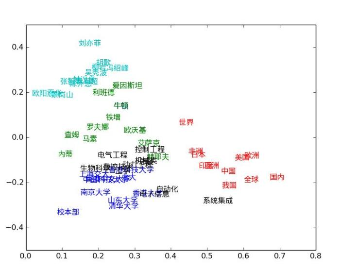
- 静态表示:Word2Vec 等预训练词向量是固定的,无法根据上下文动态调整
- 多义词困扰:同一个词在不同语境中的含义无法区分
- 上下文缺失:无法充分利用句子级别的语义信息
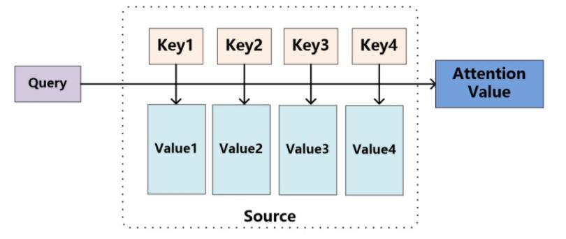
注意力机制(Attention Mechanism)
注意力机制的核心思想
注意力机制模拟人类的注意力过程,让模型能够动态地关注输入序列中的重要部分,而不是平等对待所有信息。
Self-Attention(自注意力)
基本概念
Self-Attention 是指序列内部元素之间的注意力计算,每个位置都可以关注序列中的任意位置,包括自身。
经典例子:
- "The animal didn’t cross the street because it was too tired." → "it"指向"animal"
- "The animal didn’t cross the street because it was too narrow." → "it"指向"street"
数学计算过程
Link:注意力机制的本质|Self-Attention|Transformer|QKV 矩阵哔哩哔哩 bilibili
对于输入序列
生成 Q、K、V 矩阵:
其中
是可学习的权重矩阵 计算注意力得分:
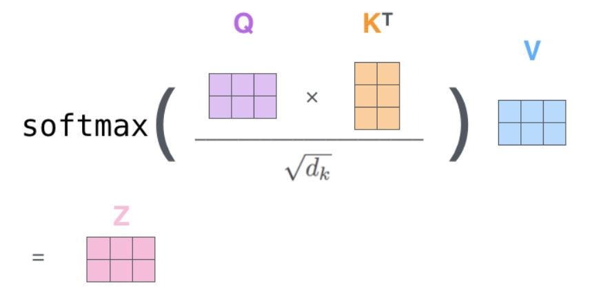
缩放因子:
用于防止点积过大导致 softmax 饱和
Self-Attention 计算流程图
graph LR
    A["输入序列 X<br/>Input Sequence<br/>n×d"] --> B["线性变换<br/>Linear Transform<br/>生成Q,K,V"]
    B --> C["查询矩阵 Q<br/>Query Matrix<br/>n×d_k"]
    B --> D["键矩阵 K<br/>Key Matrix<br/>n×d_k"]
    B --> E["值矩阵 V<br/>Value Matrix<br/>n×d_v"]

    C --> F["矩阵乘法<br/>Matrix Multiply<br/>QK^T"]
    D --> F
    F --> G["缩放处理<br/>Scale<br/>/√d_k"]
    G --> H["Softmax<br/>归一化<br/>注意力分布"]
    H --> I["注意力权重<br/>Attention Weights<br/>概率分布"]

    I --> J["加权求和<br/>Weighted Sum<br/>Attention×V"]
    E --> J
    J --> K["输出特征<br/>Output Features<br/>上下文表示"]

    style A fill:#3F51B5,stroke:#303F9F,stroke-width:3px,color:#fff
    style B fill:#FF9800,stroke:#F57C00,stroke-width:3px,color:#fff
    style C fill:#4CAF50,stroke:#43A047,stroke-width:3px,color:#fff
    style D fill:#E91E63,stroke:#C2185B,stroke-width:3px,color:#fff
    style E fill:#9C27B0,stroke:#7B1FA2,stroke-width:3px,color:#fff
    style F fill:#FF5722,stroke:#E64A19,stroke-width:3px,color:#fff
    style G fill:#607D8B,stroke:#455A64,stroke-width:3px,color:#fff
    style H fill:#FFC107,stroke:#FF8F00,stroke-width:3px,color:#333
    style I fill:#2196F3,stroke:#1976D2,stroke-width:3px,color:#fff
    style J fill:#8BC34A,stroke:#689F38,stroke-width:3px,color:#fff
    style K fill:#F44336,stroke:#E53935,stroke-width:3px,color:#fff

    linkStyle 0 stroke:#FF6B6B,stroke-width:3px
    linkStyle 1 stroke:#FF6B6B,stroke-width:3px
    linkStyle 2 stroke:#4ECDC4,stroke-width:3px
    linkStyle 3 stroke:#45B7D1,stroke-width:3px
    linkStyle 4 stroke:#96CEB4,stroke-width:3px
    linkStyle 5 stroke:#FFEAA7,stroke-width:3px
    linkStyle 6 stroke:#DDA0DD,stroke-width:3px
    linkStyle 7 stroke:#98D8C8,stroke-width:3px
    linkStyle 8 stroke:#FFB347,stroke-width:3px
    linkStyle 9 stroke:#87CEEB,stroke-width:3px
    linkStyle 10 stroke:#F7DC6F,stroke-width:3px
    linkStyle 11 stroke:#BB8FCE,stroke-width:3px
![]()
Self-Attention 的优势
- 并行计算:所有位置可以同时计算,不存在顺序依赖
- 长距离依赖:任意两个位置之间可以直接建立连接
- 动态权重:根据上下文动态调整注意力权重
Multi-Head Attention(多头注意力)
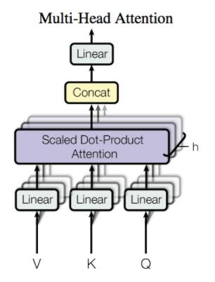
设计动机
单个注意力头可能只关注某种特定的模式,多头注意力允许模型同时关注不同子空间的信息。
位置编码
Transformer 引入了位置编码,将输入序列中的位置信息编码为向量,并作为输入序列的输入。
位置编码的计算公式为:
其中
计算公式
其中每个头:
Multi-Head Attention 架构图
graph LR
    A["输入<br/>Q,K,V<br/>查询键值"] --> B1["注意力头 1<br/>Head 1<br/>WQ1,WK1,WV1"]
    A --> B2["注意力头 2<br/>Head 2<br/>WQ2,WK2,WV2"]
    A --> B3["注意力头 3<br/>Head 3<br/>WQ3,WK3,WV3"]
    A --> B4["注意力头 h<br/>Head h<br/>WQh,WKh,WVh"]

    B1 --> C1["Self-Attention 1<br/>独立注意力计算<br/>子空间特征1"]
    B2 --> C2["Self-Attention 2<br/>独立注意力计算<br/>子空间特征2"]
    B3 --> C3["Self-Attention 3<br/>独立注意力计算<br/>子空间特征3"]
    B4 --> C4["Self-Attention h<br/>独立注意力计算<br/>子空间特征h"]

    C1 --> D["特征拼接<br/>Concatenate<br/>多头特征融合"]
    C2 --> D
    C3 --> D
    C4 --> D

    D --> E["线性变换<br/>Linear W^O<br/>输出投影"]
    E --> F["最终输出<br/>Multi-Head Output<br/>综合表示"]

    style A fill:#3F51B5,stroke:#303F9F,stroke-width:3px,color:#fff
    style B1 fill:#FF9800,stroke:#F57C00,stroke-width:3px,color:#fff
    style B2 fill:#4CAF50,stroke:#43A047,stroke-width:3px,color:#fff
    style B3 fill:#E91E63,stroke:#C2185B,stroke-width:3px,color:#fff
    style B4 fill:#9C27B0,stroke:#7B1FA2,stroke-width:3px,color:#fff
    style C1 fill:#FF5722,stroke:#E64A19,stroke-width:3px,color:#fff
    style C2 fill:#607D8B,stroke:#455A64,stroke-width:3px,color:#fff
    style C3 fill:#FFC107,stroke:#FF8F00,stroke-width:3px,color:#333
    style C4 fill:#2196F3,stroke:#1976D2,stroke-width:3px,color:#fff
    style D fill:#8BC34A,stroke:#689F38,stroke-width:3px,color:#fff
    style E fill:#795548,stroke:#5D4037,stroke-width:3px,color:#fff
    style F fill:#F44336,stroke:#E53935,stroke-width:3px,color:#fff

    linkStyle 0 stroke:#FF6B6B,stroke-width:3px
    linkStyle 1 stroke:#4ECDC4,stroke-width:3px
    linkStyle 2 stroke:#45B7D1,stroke-width:3px
    linkStyle 3 stroke:#96CEB4,stroke-width:3px
    linkStyle 4 stroke:#FFEAA7,stroke-width:3px
    linkStyle 5 stroke:#DDA0DD,stroke-width:3px
    linkStyle 6 stroke:#98D8C8,stroke-width:3px
    linkStyle 7 stroke:#FFB347,stroke-width:3px
    linkStyle 8 stroke:#87CEEB,stroke-width:3px
    linkStyle 9 stroke:#F7DC6F,stroke-width:3px
    linkStyle 10 stroke:#BB8FCE,stroke-width:3px
    linkStyle 11 stroke:#FF9999,stroke-width:3px
    linkStyle 12 stroke:#85C1E9,stroke-width:3px
    linkStyle 13 stroke:#F8C471,stroke-width:3px
参数说明
:注意力头的数量(通常为 8 或 16) :第 个头的投影矩阵 :输出投影矩阵 - 通常设置
,保证参数量不变
Cross Attention(交叉注意力)
基本概念
Cross Attention 是注意力机制的一种变体,与 Self-Attention 的主要区别在于:
- Self-Attention:Query、Key、Value 都来自同一个序列
- Cross Attention:Query 来自一个序列,Key 和 Value 来自另一个序列
计算公式
其中:
(来自序列 1) (来自序列 2) (来自序列 2)
应用场景
1. 机器翻译
- Query:目标语言的词向量
- Key & Value:源语言的词向量
- 作用:目标语言的每个词都能关注到源语言的相关词汇
2. Transformer Decoder
- Query:来自 Decoder 的隐藏状态
- Key & Value:来自 Encoder 的输出
- 作用:Decoder 在生成时能够关注到 Encoder 的全部信息
3. 图像描述生成
- Query:文本序列的隐藏状态
- Key & Value:图像的特征向量
- 作用:生成文本时关注图像的相关区域
Cross Attention 架构图
graph TB
    A["序列1 (Query源)<br/>Target Sequence<br/>n×d"] --> B["线性变换 WQ<br/>Query Transform"]
    C["序列2 (Key&Value源)<br/>Source Sequence<br/>m×d"] --> D["线性变换 WK<br/>Key Transform"]
    C --> E["线性变换 WV<br/>Value Transform"]

    B --> F["Query 矩阵<br/>Q: n×d_k"]
    D --> G["Key 矩阵<br/>K: m×d_k"]
    E --> H["Value 矩阵<br/>V: m×d_v"]

    F --> I["矩阵乘法<br/>QK^T<br/>n×m"]
    G --> I
    I --> J["缩放 & Softmax<br/>注意力权重<br/>n×m"]
    J --> K["加权求和<br/>Attention×V"]
    H --> K
    K --> L["输出特征<br/>n×d_v<br/>跨序列表示"]

    style A fill:#3F51B5,stroke:#303F9F,stroke-width:3px,color:#fff
    style C fill:#E91E63,stroke:#C2185B,stroke-width:3px,color:#fff
    style F fill:#4CAF50,stroke:#43A047,stroke-width:3px,color:#fff
    style G fill:#FF9800,stroke:#F57C00,stroke-width:3px,color:#fff
    style H fill:#9C27B0,stroke:#7B1FA2,stroke-width:3px,color:#fff
    style L fill:#F44336,stroke:#E53935,stroke-width:3px,color:#fff
与 Self-Attention 的对比
| 特性 | Self-Attention | Cross Attention |
|---|---|---|
| Q, K, V 来源 | 同一序列 | 不同序列 |
| 注意力矩阵大小 | n×n | n×m |
| 主要用途 | 序列内部建模 | 序列间关系建模 |
| 典型应用 | 语言理解、特征提取 | 机器翻译、多模态融合 |
实际应用示例
机器翻译中的 Cross Attention
源语言: "I love you"
目标语言: "我 爱 你"

Cross Attention 让:
- "我" 主要关注 "I"
- "爱" 主要关注 "love"
- "你" 主要关注 "you"
优势特点
- 跨模态连接:能够建立不同序列/模态之间的联系
- 信息融合:有效整合来自不同源的信息
- 对齐能力:在翻译等任务中实现源-目标对齐
- 灵活性:适用于各种序列到序列的任务
Cross Attention 是 Transformer 架构中实现编码器-解码器信息交互的关键机制,使得模型能够在生成过程中充分利用输入信息。